In part 2 of this series on causal inference, we introduced the idea of pair matched experimental designs and we derived Rosenbaum’s naive model. We briefly discussed the challenges of finding an optimal set of matched pairs and introduced the idea of propensity scores to simplify the pair matching process.
In this third post, we will have all of our matched pairs chosen. The next task in our observational study design will be to analyze the results. To accomplish this, we’ll take a deep dive into Wilcoxon’s signed rank test, a statistical test that is frequently used in randomized experiments and observational studies alike. Wilcoxon’s test is one of many options, and we discuss it here because it is reasonably reliable and it has many convenient properties that we will want to exploit.
Analyzing Results with Wilcoxon’s Signed Rank Test
Once the matched pairs have been obtained, we can begin the work of measuring potential treatment effects. For each pair \(p\), let \(r_{C}^p\) and \(r_T^p\) denote the responses of the control subject and the treated subject in pair \(p\). Next, let \(Y_p = r_T^p - r_C^p\) so that the vector \(\mathbf{Y} = [Y_1, Y_2, \ldots, Y_I]\) represents each of the treatment minus control response differences for all of the \(I\) pairs. To test Fisher’s hypothesis of no effect, we could set \(H_0: \mathbf{Y} = \mathbf{0}\) and \(H_a: \mathbf{Y} > \mathbf{0}\), where the inequality operator represents component wise inequality. There are a number of statistical tests that would be suitable for these hypotheses, but a popular choice is the Wilcoxon Signed Rank Test.
One reason that Wilcoxon’s test is popular is because it is nonparametric, meaning it makes no underlying assumptions about the distribution of \(\mathbf{Y}\). Although computing exact \(p\)-values from Wilcoxon’s test can be impractical for large quantities of matched pairs, its test statistic lends itself well to Normal approximation.
Test Procedure
Assuming that all the \(Y_i\) have distinct, non-zero absolute value (\(\vert Y_i \vert \neq \vert Y_j \vert\) and \(\vert Y_i \vert \neq 0\) for all \(i, j \in \{1, 2, \ldots I \}\)), the procedure for Wilcoxon’s signed rank test is as follows:
- For each \(Y_i\), compute \(\vert Y_i \vert\).
- Assign ascending ranks to the \(\vert Y_i \vert\) so that the smallest \(\vert Y_i \vert\) has \(R_i = 1\) and the largest \(\vert Y_i \vert\) has \(R_i = I\).
- Define \(U_i = 1\) when \(Y_i > 0\) and \(U_i = 0\) when \(Y_i < 0\).
- The test statistic is given by \(T = \sum_{i = 1}^I R_i U_i\).
Here, we treat the \(U_i\) as independent and identically distributed random variables with probability density function
\[p_{U_i}(Y_i) = \begin{cases} 1/2, Y_i > 0 \\ 1/2, Y_i < 0\end{cases}. \\\]One way to interpret this, and the way that Wilcoxon described it in his paper Individual Comparisons by Ranking Methods, is that we are testing the null hypothesis that the \(Y_i\) are normally distributed and centered at a mean of \(0\). The events \(Y_i < 0\) and \(Y_i > 0\) are equally likely.
Exact p-values for Wilcoxon’s Test
The \(p\)-value of Wilcoxon’s test is the probability of obtaining a test statistic \(T\) as or more extreme when the null hypothesis is true. As an example, suppose we wish to run Wilcoxon’s test on an extremely small set of \(I = 5\) pairs where
\[\mathbf{Y} = [-1.5, 3, 7.5, -9, 14].\]The \(Y_i\) are already sorted by magnitude and so the \(R_i\) are given by
\[\mathbf{R} = [1, 2, 3, 4, 5].\]The ranks associated with positive \(Y_i\) are \(2, 3,\) and \(5\), so the test statistic is \(T = 2 + 3 + 5 = 10\). Supposing that every distinct configuration of positive ranks is equally likely, what is the probability of obtaining a test statistic \(T\) as or more extreme than \(T = 10\)? Since there are \(I = 5\) pairs and each pair can be associated with either a negative or positive \(Y_i\), there are \(2^5 = 32\) possible configurations of positive ranks. Each configuration is expressed in the following table.
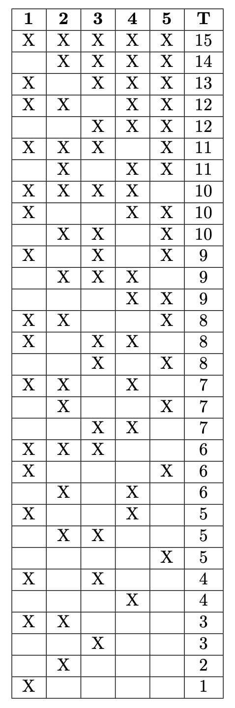
From the table, we can see that there are \(10\) distinct configurations of positive associated ranks that would lead to a test statistic \(T >= 10\). Since there are \(32\) total distinct configurations, the \(p\)-value is \(10/32 = 0.3125\).
Approximate p-values for Wilcoxon’s Test
Computing the exact \(p\)-value in this instance was simple because \(I\) is very small, but suppose we had a trial with \(I = 200\) pairs. This leads to approximately \(1.607 \times 10^{60}\) distinct configurations of positive associated ranks and so computing the \(p\)-value quickly becomes an extremely computationally expensive task. Luckily, it is straight forward to obtain a reasonably accurate estimate using normal approximations. Using the Central Limit Theorem, we have that as \(I \rightarrow \infty,\)
\[\frac{T - \mathbb{E}[T]}{\sqrt{\text{Var}[T]}} \xrightarrow{d} \mathcal{N}(0, 1).\]This approximation is reasonably accurate when \(I > 30\). We only need to compute \(\mathbb{E}[T]\) and \(\text{Var}[T]\) to use this approximation.
\[\mathbb{E}[T] = \mathbb{E}\left[ \sum_{i = 1}^I R_i U_i \right] = \sum_{i = 1}^I i \mathbb{E}[U_i] = \frac{1}{2} \sum_{i = 1}^I i = \frac{I(I+1)}{4}.\]Here we use that \(\mathbb{E}[U_i] = 1/2\) and \(\sum_{i = 1}^n i = \frac{n(n + 1)}{2}\). In deriving the variance next, we will use the independence of the \(U_i\) to say that the variance of the sum of the \(U_i\) is the sum of the variances of the \(U_i\).
\[\text{Var}[T] = \text{Var} \left[ \sum_{i = 1}^I R_i U_i \right] = \sum_{i = 1}^I i^2 \text{Var}[U_i] = \frac{1}{4} \frac{I(I+1) (2I+1)}{6} = \frac{I (I + 1) (2I + 1)}{24}.\]Here we use that \(\text{Var}[U_i] = 1/4\) and \(\sum_{i = 1}^n i^2 = \frac{n (n + 1) (2n + 1)}{6}\). In the derivation of both the expectation and the variance, we also replaced \(R_i\) with \(i\) which amounts to a simple re-indexing of the \(i\) in ascending order of the \(R_i\) and so this does not change the result in any material way.
Plugging these results into the normal approximation above, the approximate \(p\)-value is given by
\[1 - \Phi\left( \frac{T - \mathbb{E}[T]}{\sqrt{\text{Var}[T]}} \right),\]where \(\Phi\) is the cumulative distribution function of the standard normal distribution.
The test can be adjusted to accommodate for situations where there are \(i\) and \(j\) such that \(Y_i = 0\) or \(Y_i = Y_j\). In this observational study, we will be working with continuous treatment responses and so ties will not be a concern, but there will be some instances where \(Y_i = 0\). In this case, those pairs were excluded from the trial and \(R_i = 1\) was assigned to the \(Y_i\) of least non-zero magnitude.
Doses
Often within the context of an observational study, treatment dose may have varied across subjects. In response, the researcher may wish to modify Wilcoxon’s test to weigh positive associated ranks by the dose associated with that \(Y_i\).
Weighting Wilcoxon’s test with treatment doses is relatively straight forward. Let \(d_i\) denote the treatment dose associated with the treated subject in pair \(i\). The same procedure for ranking is followed but when computing the test statistic, we instead compute \(T_{\text{dose}} = \sum_{i = 1}^I R_i U_i d_i\). In doing this, ranks associated with higher doses receive more weight.
In order to make practical use of \(T_{\text{dose}}\), we need to compute \(\mathbb{E}[T_{\text{dose}}]\) and \(\text{Var}[T_{\text{dose}}]\) for the normal approximation of the \(p\)-value.
\[\mathbb{E}[T_{\text{dose}}] = \mathbb{E}\left[ \sum_{i = 1}^I R_i U_i d_i \right] = \sum_{i = 1}^I \mathbb{E}\left[ i U_i d_i \right] = \sum_{i = 1}^I i d_i \mathbb{E}[U_i] = \frac{1}{2} \sum_{i = 1}^I i d_i\] \[\text{Var}[T_{\text{dose}}] = \text{Var}\left[ \sum_{i = 1}^I R_i U_i d_i \right] = \sum_{i = 1}^I i^2 d_i^2 \text{Var}[U_i] = \frac{1}{4} \sum_{i = 1}^I i^2 d_i^2.\]Computing an exact \(p\)-value for the dose weighted test is similar to the standard Wilcoxon test except that in computing the test statistic \(T_{\text{dose}}\) for each configuration of positive associated ranks, the dose weighted sum should be used in determining whether the configuration produces a test statistic as or more extreme than \(T_{\text{dose}}\).
What’s Next
In the next installment of this series, we’ll discuss how to measure power in an observational study, and this discussion will lead us into the topic of design sensitivity. This is a sort of metric that tells us how our study’s design holds up to varying factors of bias.
Notice that in this post, we didn’t discuss any of the issues we identified in the last post related to unobserved bias. As a reminder, we cannot simply plug our results into Wilcoxon’s test and interpret our findings in an observational study because that would only be appropriate if the naive model were really true. In practice, this is extremely unlikely! We therefore need additional tools to tackle unobserved bias and obtain meaningful interpretations of our results, and so this will be the main subject matter of the next post.