In part 3, we covered Wilcoxon’s signed rank test in detail, and we did this because it is a common choice of test in observational studies due to some convenient properties. It’s easy to approximate p-values with Wilcoxon’s test using normal approximations and it’s nonparametric, so we aren’t making any assumptions about the underlying distribution of our data.

In the final installment of this series on introductory causal inference, I’ll introduce the concept of power in observational studies. Power means something different from power in typical statistical inference since there is some level of unobserved bias that we must account for.

Design Sensitivity

The \(p\)-values obtained from Wilcoxon’s Signed Rank Test from the previous section have meaningful interpretations on their own when the \(Y_i\) are obtained in a randomized experiment, but in an observational study, this would only be the case if the naive model were true. That is to say, if subjects that looked comparable were truly comparable and there were no unobserved biases across the treatment and control groups, the \(p\)-value obtained through Wilcoxon’s test could be compared to some significance level \(\alpha\) and we could decide whether there is strong evidence against Fisher’s hypothesis of no effect.

Since this is an observational study and we cannot rely on the useful properties of randomization, the \(p\)-value cannot be interpreted this way. We need a way of measuring the study’s robustness under the bias introduced by differing treatment assignment probabilities and unobserved covariates. The sensitivity analysis and design sensitivity can help us understand whether our findings hold up under varying factors of bias.

In describing the sensitivity analysis, we’ll follow Rosenbaum’s derivations in Design of Observational Studies. Recall that in the naive model, we say that subjects which appear comparable are truly comparable. That is, for two subjects \(k\) and \(l\) where \(\mathbf{x}_k = \mathbf{x}_l\), the probabilities of treatment are equal (\(\pi_k = \pi_l\)). To quantify departures from the naive model, we can use the parameter \(\Gamma \geq 1\). Suppose that for these two subjects \(k\) and \(l\), the odds of treatment differ by at most this parameter. Formally, when \(\mathbf{x}_k = \mathbf{x}_l\),

Notice that when \(\Gamma = 1\), this is equivalent to the naive model since \(\pi_k = \pi_l\). As \(\Gamma\) increases, we can represent larger and larger departures from the naive model and, in doing so, consider situations with greater and greater degrees of unobserved bias. For example, if \(\Gamma = 3\), then we would be considering the scenario where one subject (say, \(\pi_k = 3/4\)) is up to three times more likely to receive treatment than the other subject (say, \(\pi_l = 1/4\)).

Now supposing that the subjects \(k\) and \(l\) belong to one matched pair where exactly one is assigned treatment, we have that

Converting the first expression from odds ratios to probabilities and plugging this in, we obtain

This is a helpful representation of the design sensitivity model specifically for matched pair designs. Again, observe what happens as \(\Gamma\) varies. When \(\Gamma = 1\), we are back to a randomized experiment where \(\pi_k = \pi_l\). As \(\Gamma\) increases, we are considering scenarios that are larger and larger departures from the naive model in the form of unobserved bias up to a factor of \(\Gamma\).

Now that we have a method of quantifying unobserved bias, we can see how it can potentially impact the results produced by Wilcoxon’s test. Let \(\overline{\overline{T}}\) be defined as the sum of \(I\) independent random variables, \(i = 1, 2, \ldots, I\), which take the value \(i\) with probability \(\Gamma/(1 + \Gamma)\) or the value \(0\) with probability \(1/(1 + \Gamma)\). Also, let \(\overline{T}\) be defined as the sum of \(I\) independent random variables, \(i = 1, 2, \ldots, I\), which take the value \(i\) with probability \(1/(1 + \Gamma)\) or the value \(0\) with probability \(\Gamma/(1 + \Gamma)\).

Given some choice of \(\Gamma \geq 1\), following the same normal approximation procedure covered earlier on \(\overline{T}\) and \(\overline{\overline{T}}\) respectively produces lower and upper bounds on the \(p\)-value when the hypothesis test is subjected to unobserved bias up to a factor of \(\Gamma\). This is because in the null hypothesis of Wilcoxon’s test, we assume that the matched pair differences \(Y_i\) are normally distributed and centered around a mean of \(0\). In other words, it is equally likely for \(Y_i\) to be positive or negative when the null hypothesis is true. With the modified test statistics \(\overline{T}\) and \(\overline{\overline{T}}\), we are introducing a factor of bias \(\Gamma\) and thinking about how this bias might impact the test statistic.

Power in Randomized Experiments

The power of a statistical test is the probability that the null hypothesis is correctly rejected when it is false. Given some significance level \(\alpha\) and some assumed distribution \(F(\cdot)\) of \(\mathbf{Y}\), we could compute the approximate power of Wilcoxon’s test under the naive model, i.e. when \(\Gamma = 1\), by finding \(\mathbb{P}(T \geq \zeta_\alpha \vert \mathbf{Y} > \mathbf{0})\), where \(\zeta_\alpha\) is such that

If \(\Phi^{-1}\) is the quantile function of the standard normal distribution (e.g., if \(\Phi(1.645) = 0.95\). then \(\Phi^{-1}(0.95) = 1.645\)), then \(\zeta_\alpha\) is explicitly given by

Since we have already explicitly computed the expectation and variance of \(T\) in Wilcoxon’s test given that Fisher’s hypothesis is true, we can consider an example where there are \(I = 500\) pairs and \(\alpha = 0.05\):

This means that under the naive model, we would reject Fisher’s hypothesis if \(T\) were at least \(67,942\). Now that we have a critical value, we can turn our attention to expressing the power in a closed form. There is no analytic solution to compute \(\mathbb{P}(T \geq \zeta_\alpha \vert \mathbf{Y} > \mathbf{0})\) unless an assumption is made about the distribution of \(\mathbf{Y}\), so let us assume that \(Y_i \sim_{iid} F(\cdot)\). Erich Lehmann developed a method for approximating the power of Wilcoxon’s test which is as follows: set \(p = \mathbb{P}(Y_i > 0), p'_1 = \mathbb{P}(Y_i + Y_{i'} > 0)\), and \(p'_2 = \mathbb{P}(Y_i + Y_{i'} > 0, Y_i + Y_{i''} > 0)\) where \(i < i' < i''\). Then the expectation and the variance of the Wilcoxon test’s statistic \(T\) given that the null hypothesis is false are given by

Using \(\mu_F\) and \(\sigma^2_F\) in a normal approximation, we have that

If \(Y_i \sim_{iid}F(\cdot) = \mathcal{N}(\tau, \omega^2)\), we can derive exact expressions for \(p\) and \(p'_1\) and we can simulate \(p'_2\). In particular,

\(p'_1 = \mathbb{P}(Y_i + Y_{i'} > 0) = \int_{0}^{\infty} \frac{1}{2\omega \sqrt{\pi}} \exp\left\{- \frac{1}{2} \left(\frac{x - 2\tau}{\sqrt{2}\omega}\right)^2 \right\} dx = 1 - \Phi \left( \frac{-\sqrt{2}\tau}{\omega}\right).\) In the second equation, we use the property that when \(Y_i \sim \mathcal{N}(\tau_i, \sigma^2_i)\) and \(Y_{i'} \sim \mathcal{N}(\tau_{i'}, \sigma^2_{i'})\), it follows that \(Y_i + Y_{i'} \sim \mathcal{N}(\tau_i + \tau_{i'}, \sigma^2_i + \sigma^2_{i'})\).

To simulate \(p'_2\), we can take three large samples of equal size from \(\mathcal{N}(\tau, \omega^2)\), set them side by side, and report back the proportion of rows where the sum of the first and second samples and the sum of the first and third samples is strictly positive. For example, we could quickly do this in R with the following code:

# Set the mean and standard deviation of the assumed distribution of Y_i
tau <- 1/4
omega <- 1

# Sample one million random variables from the distribution three times
sample1 <- rnorm(1000000, mean = tau, sd = omega)
sample2 <- rnorm(1000000, mean = tau, sd = omega)
sample3 <- rnorm(1000000, mean = tau, sd = omega)

# Arrange the samples side by side and flag the appropriate rows
result <- data.frame(sample1, sample2, sample3)
result <- 
  result %>% 
  mutate(flag = ifelse(sample1 + sample2 > 0 & sample1 + sample3 > 0, 1, 0))

# Return the proportion of rows which were flagged, should be close to 0.482
nrow(result %>% filter(flag == 1))/nrow(result)

We now have all the required mechanics in place to generate a reasonably accurate estimation of the power of Wilcoxon’s test. This approximation of the power has a meaningful interpretation for randomized experiments. Of course, since we are dealing with observational studies, it would be useful to have an analogous interpretation of power which accounts for factors of unobserved bias \(\Gamma\) that are strictly greater than \(1\). To this end, we can consider the power of the sensitivity analysis.

Power in Observational Studies

In an observational study, we are interested in more than just the power of the statistical test used to analyze the results. We want to know what the test’s power is when the design is subjected to a factor of bias \(\Gamma\) strictly greater than \(1\). This type of power is referred to as the power of the sensitivity analysis and is computed in a similar way to the power of the statistical test. First, given a significance level \(\alpha\) and a factor of bias \(\Gamma\), we find the critical value \(\zeta_{\alpha, \Gamma}\) such that \(\mathbb{P}(T \geq \zeta_{\alpha, \Gamma} \vert \mathbf{Y} > \mathbf{0}) \leq \alpha\). Then, this critical value can be plugged into the same power approximation derived above, that is, the approximate power of the sensitivity analysis subject to unobserved bias up to a factor of \(\Gamma\) with significance \(\alpha\) is given by

Deriving the critical value \(\zeta_{\alpha, \Gamma}\) is also quite similar to deriving \(\zeta_\alpha\). We follow the same procedure except we replace \(T\) with \(\overline{\overline{T}}\). Formally,

Notice that \(\zeta_{\alpha, 1} = \zeta_\alpha\) since \(\Gamma = 1\) represents a randomized experiment and the naive model. Finally, to obtain the power of the sensitivity analysis under a factor of bias \(\Gamma\), we can plug this approximate critical value into Lehmann’s power approximation from the previous section.

A Numerical Example of Sensitivity Analysis Power Computations

In this section, we’ll reproduce one of Rosenbaum’s numerical examples of the sensitivity analysis power computations. Suppose we are conducting an observational study on \(I = 100\) matched pairs with a significance level of \(\alpha = 0.05\). We assume that \(Y_i \sim_{iid} \mathcal{N}(0.5, 1)\). Plugging these details into our approximations, we have that \(p = 0.691\), \(p'_1 = 0.76\), and \(p'_2 = 0.634\). Plugging these probabilities into the approximations of \(\mu_F\) and \(\sigma^2_F\), we have that \(\mu_F = 3832.383 \text{ and } \sigma^2_F = 56996.48\). From this, the critical value is \(\zeta_{0.05} = 3003.388\) and the approximate power of the test is

In this case, provided that the assumed distribution for \(Y_i\) is correct, we could expect the test to reject the null hypothesis when it’s false with near certainty. Notice how this result changes when we compute the power of the sensitivity analysis subject to a factor of bias \(\Gamma = 2\). In this case, the critical value \(\zeta_{0.05, 2} = 3817.695\) and yields approximate power

Defining Design Sensitivity

The discussion of the power of the sensitivity analysis so far has yielded reliable methods to approximate the power of Wilcoxon’s test under a variety of situations. We can approximate the power of this test under the naive model and we can also approximate power under varying factors of bias. This ultimately informs the concept of the design sensitivity.

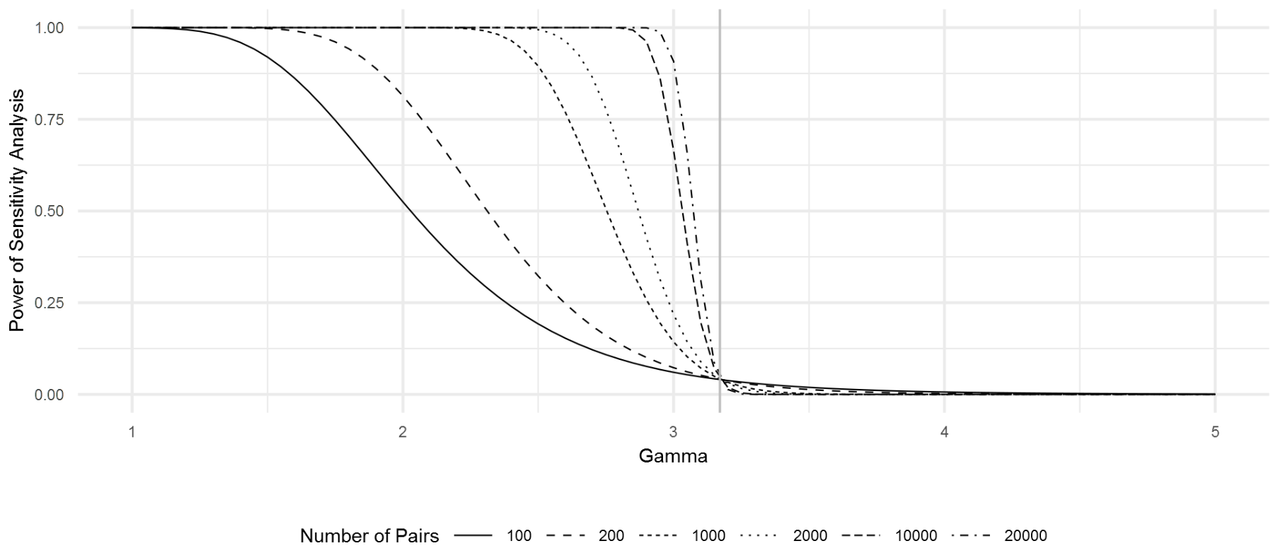
Observe the plot of \(\Gamma\) against power of the sensitivity analysis reproduced from Rosenbaum in the figure below. Each line represents a different number of pairs in the sample. We can see that as \(I \rightarrow \infty\), the power of the sensitivity analysis tends toward \(1\) when \(\Gamma < 3.171\) and tends toward \(0\) when \(\Gamma > 3.171\). This point \(\widetilde{\Gamma} = 3.171\) is called the design sensitivity.

The design sensitivity is the parameter best suited for evaluating the quality of a particular experimental design. Thinking back to the standard Wilcoxon statistic and the dose weighted statistic, we could make a decision on which is the best choice by looking at which one produces a higher design sensitivity.

Rosenbaum provides a theorem with proof describing the relationship between the power of the sensitivity analysis and the design sensitivity, and he also provides a formula for the design sensitivity of the standard Wilcoxon test statistic.

Of course, this all depends on the choice of distribution for the \(Y_i\), and so care must be taken to ensure that the distribution is estimated well.

Final Thoughts

Throughout this series of posts, we’ve examined a lot of complex ideas from causal inference. This subject is what I wrote my master’s project on and I believe that it is ripe for many new discoveries and interesting applications across all industries. In particular, I’m excited to learn more about how these ideas can be applied in medicine, recommendation engines, and finance.