Decision trees have long been part of the machine learning toolkit. They can be very effective as classifiers, especially when several decision trees are combined together in an ensemble learning algorithm. In this article, which is the first of a series on decision tree algorithms, we’ll cover one of the earliest methods of building a decision tree: the Iterative Dichotomiser 3 (ID3) algorithm. This algorithm is a recursive process that builds decision trees by maximizing a quantity called information gain at each branch. Once the desired depth is obtained for a particular branch, a “leaf” is attached to denote how the model would classify matching data points. We’ll cover this process in great detail throughout this article. As usual, we’ll also walk through an unoptimized implementation of the ID3 algorithm in Python. The implementation is strictly to deepen understanding of the algorithm; there are much better, optimized libraries out there to build decision trees in a production environment!
This post has a GitHub repository!
This topic requires no advanced mathematics; a good understanding of college level algebra is sufficient to understand the ID3 algorithm. In the sections about implementing the algorithm in Python, the reader is assumed to have familiarity with basic Python concepts like loops and classes.
Table of Contents
- Table of Contents
- What are decision trees?
- The ID3 Algorithm
- Python Implementation of ID3
- Conclusion
What are decision trees?
Before diving into the ID3 algorithm, it’s important to understand the type of model the ID3 algorithm produces, which is a decision tree. Decision trees are classification models that can be applied to a wide range of machine learning problems. The word tree is used to describe the model because they are constructed from “branches” and “leaves” that allow the user to predict some attribute about a given data point.
To illustrate this, suppose we have a list of voters from a recent local election. The voters are choosing between Candidate A and Candidate B and we know which candidate each person voted for. We also know other things about the voters, like their biological sex (Male, Female, Unspecified), marital status (Never Married, Married, Divorced, Widowed), income level (Low, Average, High), and level of education (High School, Bachelors, Graduate). We could use a decision tree algorithm to construct a tree that would allow us to predict how someone votes based on some or all of these attributes. For example, this tree is a valid decision tree for this scenario:
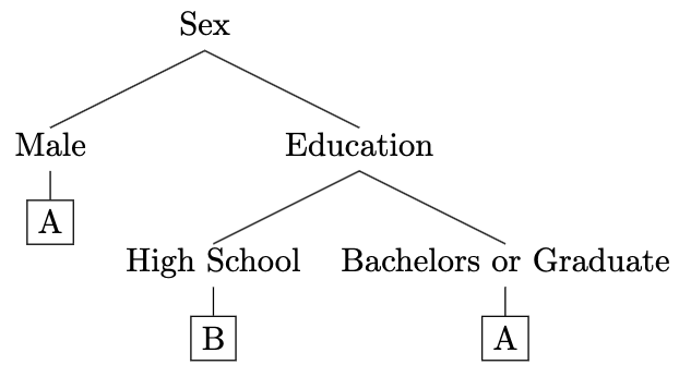
Notice that in this example, not every feature was used to predict which candidate the vote goes to. That is to say, it isn’t necessary to consider every attribute when making predictions with a decision tree. In fact, simpler trees will often outperform more complex trees.
The ID3 Algorithm
Preliminaries
Before diving head first into the ID3 algorithm, it will be useful to have some familiarity with some concepts commonly used in statistics and machine learning. Once we’ve covered these concepts, we can go straight into the algorithm and its implementation.
Entropy
The first concept is entropy, which is a metric that is used to measure the amount of uncertainty in a data set. Formally, let \(D\) denote the set of each of the labels in the training set and \(X\) denote the set of distinct labels in the training set. Suppose that \(D = \{ \text{B, A, A, A, B, } \ldots \}\); then \(X = \{ A, B \}\). Also, let \(X_i\) denote the set of labels equal to \(i\) (e.g., \(X_A = \{A, A, A, \ldots \}\)). Then the entropy is defined as
\[E(D) = \sum_{i \in X} - \frac{|X_i|}{|X|} \log_2 \left( \frac{|X_i|}{|X|} \right),\]where \(\vert \cdot \vert\) represents the number of elements in the set. For brevity, from this point on we will let \(p(i) = \vert X_i \vert / \vert X \vert\) so that
\[E(D) = \sum_{i \in X} - p(i) \log_2 p(i).\]As an example, suppose that we are working with a data set of five subjects with \(D = \{\text{A, A, B, A, B} \}\). Three of the subjects voted for candidate A and two of the subjects voted for candidate B, so
\[\begin{align*} E(D) & = \sum_{i \in X} -p(i) \log_2 p(i) \\ & = - \frac{|X_A|}{|X|} \log_2 \left( \frac{|X_A|}{|X|} \right) - \frac{|X_B|}{|X|} \log_2 \left( \frac{|X_B|}{|X|} \right) \\ & = - \frac{3}{5} \log_2 \left( \frac{3}{5} \right) - \frac{2}{5} \log_2 \left( \frac{2}{5} \right) \\ & \thickapprox 0.971. \end{align*}\]Notice what happens when \(D\) contains labels that are all the same. If \(D = \{\text{A, A, A, A, A} \}\), then
\[E(D) = -\frac{5}{5} \log_2 \left( \frac{5}{5} \right) = -\log_2(1) = 0.\]That is, when there is more certainty about the classification of the data, the entropy tends to \(0\).
\[\text{More Certainty} \iff \text{Less Entropy}\] \[\text{Less Certainty} \iff \text{More Entropy}\]The reason that entropy is relevant to our discussion of the ID3 algorithm is that it will tell the algorithm which attribute to split on. Recall the example tree from earlier:
Notice how the first attribute the tree splits on is sex. Under the ID3 algorithm, this would imply that out of sex, marital status, education, and income, splitting on sex reduced uncertainty in the resulting subsets the most.
Information Gain
The concept we just touched on is known as information gain, which is formally defined as
\[IG(D, A) = E(D) - \sum_{t \in T} \frac{|t|}{|D|} E(t) = E(D) - E(D|A),\]where \(T\) denotes the resulting subsets of labels after splitting on the attribute \(A\). For example, suppose we are working with a small data set:
| Sex | Education | Vote |
|---|---|---|
| F | B | B |
| M | B | A |
| F | B | A |
| M | B | A |
| M | G | B |
In this case, we can choose to split on either sex or education. Let’s calculate the information gain associated with splitting on each of these to decide which attribute we should split on first. To begin, we need the entropy of the entire unsplit data set:
\[E(D) = -\frac{2}{5} \log_2 \left( \frac{2}{5} \right) - \frac{3}{5} \log_2 \left( \frac{3}{5} \right) \thickapprox 0.971.\]Next, we compute \(\frac{\vert t \vert}{\vert D \vert} E(t)\) for both variables. Splitting on sex yields the following tables:
| Sex | Education | Vote |
|---|---|---|
| F | B | B |
| F | B | A |
| Sex | Education | Vote |
|---|---|---|
| M | B | A |
| M | B | A |
| M | G | B |
For the female table, we have
\[\frac{|t|}{|D|} E(t) = \frac{2}{5} \left( -\frac{1}{2} \log_2 \left( \frac{1}{2} \right) -\frac{1}{2} \log_2 \left( \frac{1}{2} \right) \right) = 0.4.\]For the male table, we have
\[\frac{|t|}{|D|} E(t) = \frac{3}{5} \left( -\frac{2}{3} \log_2 \left( \frac{2}{3} \right) -\frac{1}{3} \log_2 \left( \frac{1}{3} \right) \right) \thickapprox 0.551.\]Putting all of this together, the information gain when splitting on sex is
\[IG(D, \text{Sex}) \thickapprox 0.971 - 0.951 = 0.02.\]A similar set of calculations for the split on education yields
\[IG(D, \text{Education}) \thickapprox 0.971 - 0.649 = 0.322,\]and so in this case, splitting on education is the best choice since it yields the greatest information gain. This is exactly the set of steps that the ID3 algorithm uses in order to decide which attribute to split on at the next branch.
At this point, we’re ready to dive into the algorithm!
Algorithm Steps
Here are the steps of the ID3 algorithm in their entirety (in pseudocode). Don’t worry if something doesn’t make sense when you first read it. We’ll cover each of these steps individually in this section.
ID3(Examples, Target, Attributes):
  1. Create the root node
  2. If every example target is C:
        Set root node to a single node tree with leaf C attached
  3. Else if Attributes is empty:
        Set root node to a single node tree with leaf labelled C,
        where C is the most common value of Target in Examples
  4. Else:
      1. Set A to be the attribute that yields the highest
         information gain.
      2. For each distinct value x_i of A in Examples
          1. Create a branch connecting to the root node that
             corresponds to A = x_i
          2. Set Examples(x_i) to the subset of Examples which have
             A = x_i
          3. If Examples(x_i) is empty:
                Below the branch, attach leaf labelled C, where C
                is the most common value of Target in Examples
          4. Else:
                To the branch, connect
                ID3(Examples(x_i), Target, Attributes - {A})
  5. Return the root node
Let’s talk through all of these steps in detail.
Steps 1 - 3: Create the root node and handle edge cases
Every decision tree needs a root node. In the first iteration of the decision tree, the root will typically represent the first attribute that we split on. There are two cases where the root does not represent an attribute split. Repesenting steps 2 and 3 respectively, those cases are:
- The attribute set is empty. In this case, there are no attributes left to split on and so the root will just have one leaf attached that represents the most common target class in the examples.
- The target class for every eample is the same. In this case, the root will just have one leaf attached that represents this class.
Throughout the recursion, we will hit these steps over and over again because the ID3 algorithm works by connecting root nodes formed in deeper layers of the recursion to earlier root nodes. In this way, every node can be thought of as its own root node for its respective subtree. Look back to our small example tree from earlier:
If we go a layer deeper than the sex node, we can visualize two different trees. In the first subtree, we have a node called Male with a leaf labelled A attached. This is an example of step 2 in action. This indicates that after the algorithm split on Sex, the Male subset all had target attribute equal to A, so there is no need to continue splitting.
In the second subtree, we have a node called Education that splits between High School or Bachelors/Graduate. This indicates that in the Female subset, there was a mix of A and B target attributes and so further splitting provided additional information gain.
Finally, in the deepest layer, we can see two trees. Each has one root with one leaf attached. In both of these trees, either the step 2 or step 3 scenario is possible. That is to say, the leaves were attached because either there were no additional attributes to split on or once the split on Education occurred, the target attribute within each of the resulting example subsets was the same across all of the examples.
Step 4: Add a new split
This is the step where the magic happens and there’s a lot of moving parts here. To make understanding this step as easy as possible, we’re going to talk about each substep individually.
Step 4.1: Identify the correct attribute
This is where we apply the concepts of entropy and information gain from earlier. For every attribute in the Attributes argument, we compute the corresponding information gain. The attribute that yields the highest information gain is the attribute we split on.
Step 4.2: Attach branches for each value of the attribute
Once the proper attribute \(A\) has been selected, we attach a branch to the root node that represents every possible value of the attribute. There is an important nuance to understand regarding this step: when we say every possible value, we mean exactly that. We do not mean every distinct value of the attribute in the examples, but every possible value.
For example, think about a decision tree we could build for the election scenario. The education attribute has three possible values: High School, Bachelors, and Graduate. If the examples in this iteration of the algorithm don’t include any individuals with a graduate degree, we still need to decide what to do with people that fall into this bucket even though we have no corresponding examples in the training set. Otherwise, there will be holes in the model for certain buckets and when we want to make predictions about those buckets later, we won’t be able to.
All right, so we attach a branch to the root node that correponds to every possible value of the attribute. Steps 4.2.1 - 4.2.4 give instructions on what we do for each branch, which is as follows.
For each new branch, we define Examples(\(x_i\)) to be the subset of the examples such that \(A = x_i\). In the situation we just described where this set of examples is empty, we simply attach a leaf equal to the most common target label in the broader examples set. If the examples set is nonempty, however, we recursively create a new instance of ID3 using Examples(\(x_I\)) instead of Examples and Attributes \(- \hspace{0.15cm} \{A\}\) instead of Attributes and attach the resulting tree to the branch. In other words, we create a brand new decision tree using the subset of examples where \(A = x_i\).
Step 5: Return the root
Once every branch of the current instance of ID3 has had a leaf attached, we return the root node with all of the respective branches and leaves. The process continues for any higher level instances of ID3 in the recursion until we finally return the highest level root node with every branch and leaf attached.
Preparing for Implementation
That is the knitty gritty of the ID3 algorithm. Of course, it is much easier to understand a description of the algorithm than to successfully code it up. Implementing recursive algorithms can be particularly challenging, but never fear! We will now cover the implementation in detail.
Python Implementation of ID3
For this implementation, we will need the math and pandas packages.
import math
import pandas as pd
This unoptimized Python implementation of the ID3 algorithm will use two classes: DecisionTreeNode and DecisionTree.
DecisionTreeNode
The class DecisionTreeNode will contain only a constructor method that will contain attributes that describe everything about a particular part of the tree. Take a moment to study the constructor for DecisionTreeNode.
class DecisionTreeNode:
    def __init__(self, attribute, value, type, parent):
        self.attribute = attribute # which attribute the node is
        # giving instructions for (e.g., outlook, humidity)
        self.value = value # the value of the attribute the
        # node is giving instructions for (e.g., the outlook is //sunny//)
        self.type = type # whether the node is a root, branch,
        # or leaf
        self.parent = parent # the node's parent node
        self.child = [] # a list of nodes that this node points
        # to in the tree
        self.depth = 0 # the depth of the tree is maintained at
        # the level of each node for convenience of access
        self.most_common = None # the most common label at each
        # particular node is recorded
The constructor for a new node accepts four arguments: attribute, value, type, and parent. For each node, this allows us to keep track of what attribute (e.g., Education) the node is associated with, the value of that attribute (e.g., Graduate), what kind of node it is (root, branch, or leaf), and which node in the tree is the current node’s parent.
The parent argument is another DecisionTreeNode class object. The remaining arguments are strings. Notice too that we assign the attributes child, depth, and most_common when we create a new node. The child attribute will be a list of every node whose parent is the current node. The depth attribute will keep track of how many layers deep the node is (root depth is 0, next level down is 1, and so on). Finally, the most_common attribute will record which target label is most common in the current node’s example subset.
DecisionTree
Phew! That’s a lot of information to keep track of. We’re not done yet, though. We need another class that will contain the machinery to construct the tree. That class will be defined as follows:
class DecisionTree:
    def __init__(self, max_depth):
        self.root = DecisionTreeNode(None, None, "root", None)
        self.max_depth = max_depth
        self.node_count = 0

    def add_branch(self, parent, attribute, value):
        new_node = DecisionTreeNode(attribute, value, "branch", parent)
        new_node.parent.child.append(new_node)
        new_node.depth = new_node.parent.depth + 1
        self.node_count += 1
        return new_node

    def add_leaf(self, parent, value):
        new_leaf = DecisionTreeNode(None, value, 'leaf', parent)
        new_leaf.parent.child.append(new_leaf)
First, take a look at the constructor for the DecisionTree class. When we create a new instance, we specify a maximum depth in the max_depth argument and we get an object with three attributes.
The root attribute is a new node from our DecisionTreeNode class which has no attribute, value, or parent. This makes sense because when we create a brand new tree, we must start from the root and we haven’t decided what attributes to split on yet.
The max_depth attribute will be used to limit the depth of the tree if we want; even if there are additional attributes to split on, once our tree is max_depth layers deep, we’ll just attach leaves as if there were no more attributes to split on and call it a day.
Finally, the DecisionTree object also has an attribute node_count which will keep track of the total number of nodes in the tree.
We’ve also defined two object methods that belong to this class: add_branch() and add_leaf().
add_branch()
This method does what it sounds like: it creates a new branch and adds it to the proper parent node. Notice that this method accepts three arguments: parent, attribute, and value. With these arguments, we keep track of which node this branch attaches to from above, what attribute it corresponds to, and the value of the attribute for its respective example subset. Let’s break down the code line by line.
def add_branch(self, parent, attribute, value):
    new_node = DecisionTreeNode(attribute, value, "branch", parent)
In this first line, we create a new branch node with the DecisionTreeNode constructor. We feed all of the add_branch() arguments to this node.
new_node.parent.child.append(new_node)
Next, we need to append the newly created node to the parent node’s children list. new_node.parent.child refers to the child attribute of the new node’s parent, so we just tack on the append method with the newly created node to accomplish this task.
new_node.depth = new_node.parent.depth + 1
Next, we set the newly formed node’s depth, which we obtain by simply adding 1 to its parent’s depth attribute.
self.node_count += 1
return new_node
Last, we increment the tree’s node count by one and return our newly created node.
add_leaf()
Again, this method does what it sounds like: it adds a leaf node to the tree. This object method accepts only two arguments: parent and value. Unlike the add_branch() method, we do not need to feed the add_leaf() method an attribute argument because this node’s value argument will be the predicted target label for whatever path on the tree it represents.
The method has only two lines of code:
new_leaf = DecisionTreeNode(None, value, 'leaf', parent)
new_leaf.parent.child.append(new_leaf)
We begin by creating a new node of type leaf and then append the node to its parent’s list of children.
Supporting Functions
All right, we now have all of the machinery in place to support the data structures for decision trees. Next, we will go over the supporting functions we’ll need to build decision trees with the ID3 algorithm.
label_proportions()
We’ll use this function to get a list of the proportions for each label in the target vector.
def label_proportions(labels):
    unique_labels = []
    unique_proportions = []
    for x in labels:
        if x not in unique_labels:
            unique_labels.append(x)
    for y in unique_labels:
        unique_proportions.append(labels.count(y)/len(labels))
    return unique_proportions
We simply plug in the vector of labels from the data set and we get back a vector giving us what proportion of the vector is equal to each distinct label. We do not need to know which proportion is associated with which label because we will only use these numbers in the next function, entropy().
entropy()
We will need a function to compute the entropy of a set of labels. This function calls on label_proportions() and then calculates the entropy of the set of labels provided.
def entropy(labels):
    proportions = label_proportions(labels)
    transformed_proportions = [ -x*math.log(x, 2) for x in proportions]
    entropy = sum(transformed_proportions)
    return entropy
get_unique_values()
Next, we have a function that will retrieve every attribute’s unique values in the provided data set. This function will be used to determine how many branches need to be created when we want to add a new split to the tree.
def get_unique_values(data):
    unique_values_dict = {}
    for x in list(data.columns):
        values = []
        for y in list(data[x]):
            if y not in values:
                values.append(y)
        unique_values_dict[x] = values
    return unique_values_dict
The value of this function is a dictionary that catalogues the unique values of every column of a pandas DataFrame. The keys are the column names and the values are the unique values for the respective columns.
add_leaf_condition()
We will need a way to know when it’s time to add a leaf instead of a branch. That’s what this function does:
def add_leaf_condition(data, target, node, max_depth):

    if len(data.columns) == 1:
        return True
    elif node.depth == max_depth and max_depth > 0:
        return True
    elif len(get_unique_values(data)[target]) == 1:
        return True
    else:
        return False
There are three scenarios when a leaf should be added.
First, when there are no additional attributes to split on, which corresponds to
if len(data.columns) == 1:
    return True
If the length of the columns in our data set is 1, then all that is left is the target column, meaning there are no additional attributes to split on!
Second, we should add a leaf if the current node has a depth attribute equal to the tree’s max_depth attribute. In this case, we are forcing the algorithm to stop even if there are additional attributes in the data set that we could potentially split on. This can be helpful when we are interested in building shallow trees and in practice, we often want to produce simple trees over more complex ones because they generally perform better. This condition corresponds to
elif node.depth == max_depth and max_depth > 0:
    return True
Notice that we also include the condition max_depth > 0 in the if statement. This means that if we set the tree’s max_depth parameter to 0, we are providing no maximum depth constraint and the algorithm will run until one of the other two leaf conditions is met.
The final leaf condition is when the example subset only contains examples with the same label. In this case, further splitting is not required and we can just add a leaf corresponding to the unanimous label. This corresponds to
elif len(get_unique_values(data)[target]) == 1:
    return True
If none of these three conditions are met, the algorithm will continue splitting the data set and building out the tree.
most_common()
We need to keep track of which label is the most common for each node’s example subset because this will allow us to attach the correct labels to the leaves of the tree. This means we need a function to identify the most common label in a vector of labels. This function accomplishes that task:
def most_common(list):
    value_counts = {}
    for y in list:
        if y not in value_counts.keys():
            value_counts[y] = 1
        else:
            value_counts[y] += 1
    return max(value_counts, key = value_counts.get)
select_attribute()
This is one of our more complex supporting functions. This function will put several of the prior functions together to select the best attribute to split on.
def select_attribute(data, target):
    base_entropy = entropy(data[target])
    information_gain_dict = {}
    total_records = data.shape[0]
    unique_values_dict = get_unique_values(data)
    non_target_features = list(data.columns)
    non_target_features.remove(target)
    for x in non_target_features:
        feature_unique_values = unique_values_dict[x]
        information_gain = base_entropy
        for y in feature_unique_values:
            filtered_data_by_feature = data[data[x] == y]
            filtered_total_records = filtered_data_by_feature.shape[0]
            information_gain -= entropy(list(filtered_data_by_feature[target]))*(filtered_total_records/total_records)
        information_gain_dict[x] = information_gain
    selected_attribute = max(information_gain_dict, key = information_gain_dict.get)
    return [selected_attribute, unique_values_dict[selected_attribute]]
Let’s walk through this function a few lines at a time.
base_entropy = entropy(data[target])
information_gain_dict = {}
total_records = data.shape[0]
unique_values_dict = get_unique_values(data)
non_target_features = list(data.columns)
non_target_features.remove(target)
In these first few lines, we’re setting the stage to select the right attribute. We compute the entropy of the example labels and create a blank dictionary that will keep track of the information gain for each attribute. We record the total number of examples in the data set and the unique values for each of the example attributes. Finally, we create a list of each attribute that is not the target, which we’ll iterate through in the next chunk.
for x in non_target_features:
    feature_unique_values = unique_values_dict[x]
    information_gain = base_entropy
    for y in feature_unique_values:
        filtered_data_by_feature = data[data[x] == y]
        filtered_total_records = filtered_data_by_feature.shape[0]
        information_gain -= entropy(list(filtered_data_by_feature[target]))*(filtered_total_records/total_records)
    information_gain_dict[x] = information_gain
Listen, I’m not a software engineer, I’m a statistician. I recognize that this loop is \(O(n^2)\). Could I optimize it to be \(O(n)\)? Probably. Am I going to? Not unless someone is paying me money to do it. I am a man of limited mental and emotional energy, after all. Do as I say, not as I do.
Anywho, in this chunk, we’re going to iterate through each attribute and record the information gain. For each attribute, we set the information gain to the entropy of the broader data set and then subtract the entropy of each resulting subset of the data when we filter on each of the attribute’s unique values. Recall that the information gain is
\[IG(D, A) = E(D) - \sum_{t \in T} \frac{|t|}{|D|} E(t),\]so in doing this, we obtain precisely the information gain for the attribute once we’ve iterated through each of the attribute’s unique values. Finally, the information gain is recorded in a dictionary where the key is the attribute name and the value is information gain associated with the attribute.
selected_attribute = max(information_gain_dict, key = information_gain_dict.get)
return [selected_attribute, unique_values_dict[selected_attribute]]
The last step is easy! Our selected attribute is the one that gives us the most information gain, so we just select the key from the information gain dictionary that has the maximum value. The function finally returns a list containing the attribute name and its associated unique values.
The ID3 Recursion
We are finally ready to tackle the ID3 recursion. The recursion combines all of the supporting functions and data structures we’ve created so far. The recursion function that constructs the decision tree is as follows:
def build_tree(tree, data, target, parent):
    next_branch_attribute = select_attribute(data, target)
    for i in next_branch_attribute[1]:
      new_node = tree.add_branch(parent, next_branch_attribute[0], i)
      filter_attribute = str(new_node.attribute)
      filter_value = str(new_node.value)
      filtered_data = data[data[filter_attribute] == filter_value]
      filtered_data = filtered_data.loc[:, filtered_data.columns != new_node.attribute]
      new_node.most_common = most_common(list(filtered_data.loc[:, target]))
      if add_leaf_condition(filtered_data, target, new_node, tree.max_depth):
          tree.add_leaf(new_node, new_node.most_common)
      else:
          build_tree(tree, filtered_data, target, new_node)
Let’s walk through the recursion a few lines at a time.
def build_tree(tree, data, target, parent):
    next_branch_attribute = select_attribute(data, target)
The recursion accepts four arguments: tree, data, target, and parent.
The tree argument is an instance of the DecisionTree class from earlier. The data argument is the data set used to construct this tree or subtree. The target argument is the column name of the example labels. Finally, the parent argument is the parent node of the current subtree. Remember that the algorithm works by creating many subtrees and attaching them together, which is why need to specify where to connect each subtree.
We start the process by identifying the next attribute we wish to split on, which we accomplish via the select_attribute() function.
for i in next_branch_attribute[1]:
Recall that the select_attribute() function returns a list of two objects. The first object is the name of the attribute we want to split on. The second object is the set of all the unique values of that attribute. This for loop iterates through each of the unique values, creating a separate branch for each one. Let’s dive into the details of the loop.
new_node = tree.add_branch(parent, next_branch_attribute[0], i)
filter_attribute = str(new_node.attribute)
filter_value = str(new_node.value)
Now that we’ve selected the attribute to split on, we’re going to add a branch to our tree for each of the attribute’s unique values. We attach a branch node to the parent specified in the parent argument with the applicable attribute name and whatever unique value we’re currently iterating through. We are going to want to filter the examples down to the examples with the current attribute and unique value combination, so we save that information into the variables filter_attribute and filter_value.
filtered_data = data[data[filter_attribute] == filter_value]
filtered_data = filtered_data.loc[:, filtered_data.columns != new_node.attribute]
new_node.most_common = most_common(list(filtered_data.loc[:, target]))
Next, we create the branch’s example subset by filtering out any examples that are not associated with this branch’s applicable attribute and unique value combination. Once the filtering is done, we remove the current attribute from the example subset and record the most common label.
if add_leaf_condition(filtered_data, target, new_node, tree.max_depth):
    tree.add_leaf(new_node, new_node.most_common)
else:
    build_tree(tree, filtered_data, target, new_node)
Here is the recursive step. At this point, we have a fresh branch and we need to decide whether we are going to continue splitting or whether we are going to attach a leaf instead.
If one of the three conditions described in the add_leaf_condition() section above is met, we add the leaf and the recursion for this pathway ends.
If none of the leaf conditions are met though, we start the process over again with the pared down example subset and attach a subtree built on this subset to the branch instead. Neat!
Learning a Tree
Let’s use all of this code to finally learn a decision tree. We’re going to use a simulated data set that follows the election scenario outlined at the beginning of this article. You can find the data set here within this post’s GitHub repository. There is a training data set and test data set.
Let’s build some trees and see how we do. We will use additional functions that weren’t covered here to generate predictions and obtain accuracy metrics for our decision trees. You can view that code in the repository if you wish.
import DecisionTree as dt
import pandas as pd

tree = dt.DecisionTree(0)

data = pd.read_csv("../data/votes.csv")

train_data = pd.read_csv("../data/train_data.csv")
test_data = pd.read_csv("../data/test_data.csv")

dt.build_tree(tree, train_data, "votes", tree.root)

train_predictions = dt.get_tree_predictions(tree, train_data)
test_predictions = dt.get_tree_predictions(tree, test_data)

train_accuracy = dt.get_test_accuracy(train_data, "votes", train_predictions)
test_accuracy = dt.get_test_accuracy(test_data, "votes", test_predictions)

print("Train Accuracy: ")
print(train_accuracy)
print("Test Accuracy: ")
print(test_accuracy)

tree_md2 = dt.DecisionTree(2)

dt.build_tree(tree_md2, train_data, "votes", tree_md2.root)

train_predictions = dt.get_tree_predictions(tree_md2, train_data)
test_predictions = dt.get_tree_predictions(tree_md2, test_data)

train_accuracy = dt.get_test_accuracy(train_data, "votes", train_predictions)
test_accuracy = dt.get_test_accuracy(test_data, "votes", test_predictions)

print("Train Accuracy, Max Depth = 2: ")
print(train_accuracy)
print("Test Accuracy, Max Depth = 2: ")
print(test_accuracy)
When we run this code, we get the following accuracy metrics:
Train Accuracy:
100.0
Test Accuracy:
100.0
Train Accuracy, Max Depth = 2:
96.22857142857143
Test Accuracy, Max Depth = 2:
95.63333333333334
Not half bad, huh?
Conclusion
What a journey we’ve been on! We’ve covered so much and yet this really only scrapes the surface of what can be done with decision trees.
Decision trees are an inexpensive and often effective classification tool. As is the case with many other machine learning tools, they are prone to overfitting and so care must be taken in the training process to avoid this problem.
In a future post, I’ll discuss even more applications of decision trees. I might cover a different algorithm or discuss how many decision trees can be trained in ensemble methods like random forests or other ensemble methods.