In this article, we’ll explore the gradient descent algorithm in detail. We’ll cover the mathematical machinery behind the algorithm, how it works in practice, and cases where it’s useful and where it’s not. I’ll also demonstrate a basic, unoptimized Python implementation of gradient descent.
In a subsequent article, we’ll go over the stochastic gradient descent (SGD) algorithm that’s frequently used in machine learning. We’ll use the Python implementation from this article to run SGD on an example data set to train a classifier model and see how well it works.
Note: in order to get the most out of this article, you’ll need to have some background knowledge in calculus—particularly with regard to derivatives and gradients.
Table of Contents
- What is the Gradient Descent Algorithm?
- A Single Variable Example
- 1. Choose a convergence criterion.
- 2. Choose an initial point to start the algorithm.
- 3a. Compute the direction of steepest descent.
- 3b. Compute the first iteration.
- 4. Check for convergence.
- 5. Continue to obtain the second iteration.
- 6. Continue to obtain the third iteration.
- 7. Continue to obtain the fourth iteration.
- Practical Considerations
- A Simple Python Implementation
- Conclusion
What is the Gradient Descent Algorithm?
The gradient descent algorithm is an optimization technique that can be used to find minima of functions and the points at which these minima are attained. If we wish to find the minimum value of the function \(f(x)\), we can choose an initial point \(x_0\) to start from. Next, we find the direction of the function’s steepest descent at \(x_0\) (which is the negative gradient, \(-\nabla f(x_0)\)) and take a small step in that direction to arrive at \(x_1\). Then, we repeat this process until we’re “satisfied” with our results.
More precisely, the algorithm is given by the following steps (which we’ll examine in more detail below):
- Choose a convergence criterion \(\epsilon > 0\).
- Choose an initial point \(x_0\) to start the algorithm.
- For each iteration \(k\):
- Compute the direction of steepest descent of \(f\) at \(x_k\), denoted by \(d_{k} = - \nabla f(x_{k})\).
- Compute the next iteration \(x_{k + 1} = x_k + t_k d_k\), where \(t_k\) is a step size that could be constant or could change with each iteration.
- For each iteration \(k\), check for convergence of the algorithm:
- If \(\mid \mid x_{k + 1} - x_k \mid \mid > \epsilon\), keep going.
- If \(\mid \mid x_{k + 1} - x_k \mid \mid \leq \epsilon\), stop and return \(x_{k + 1}\) as the optimal solution and \(f(x_{k + 1})\) as the optimal value of \(f\).
A Single Variable Example
Let’s examine each of these steps in greater detail with a concrete example. Suppose we want to find the minimum value of the function \(f(x) = x^2 - 2x - 3\).
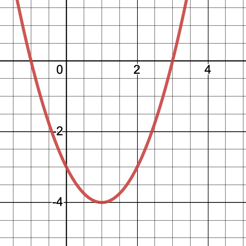
Visually, we can quickly see that the minimum value of this function is \(-4\) and that \(f\) attains that minimum value at \(x = 1\). It will be helpful to know the true solution ahead of time so we can compare our results to these values later on.
1. Choose a convergence criterion.
For this example, we’ll choose \(\epsilon = 1/8\), meaning that we’ll say the algorithm has converged on the \(k^{\text{th}}\) iteration if \(\mid \mid x_k - x_{k - 1} \mid \mid = \mid x_k - x_{k - 1}\mid \leq 1/8\). Note that \(\mid \mid x_k - x_{k - 1} \mid \mid = \mid x_k - x_{k - 1}\mid\) only because \(f\) is a single variable function in our example. In the more common multivariate case, the Euclidean norm \(\mid \mid \cdot \mid \mid\) must be used.
You may be wondering what setting a convergence criterion means exactly or what the point of setting a convergence criterion is. If you don’t care or already know, you can move onto step 2.
The plain English translation of the convergence criterion is that once the distance between two consecutive iterations is “small enough,” we’ll stop and say that the final iteration is “good enough” for us. The intuition behind this is that if consecutive iterations are only a very small distance apart, it’s likely that \(- \nabla f(x) \thickapprox \mathbf{0}\), i.e., we’re very close to a stationary point of \(f\) (and so hopefully, the optimal solution).
But if we’re interested in finding the true optimum point, why bother setting the criterion? Why not let the algorithm run until it hits the actual optimum? It turns out that there are a couple of very compelling reasons to set a convergence criterion.
First, it’s possible that for a particular problem, the gradient descent algorithm will never converge to the true optimal solution. For these cases, the algorithm may happily go on forever without ever returning an optimal value, even if its iterations become extremely close to the true optimum without ever reaching it.
Second, in practice, we’re often satsified with an answer that’s pretty close to the true optimum. To illustrate, suppose on the \(k^{\text{th}}\) iteration that \(x_k\) is within \(10^{-8}\) of the true optimum \(x^*\) (i.e., \(\mid \mid x^* - x_k \mid \mid < 10^{-8}\)). It’s possible (even likely!) that we don’t care about this small gap between the true optimum and \(x_k\) and that we’d rather just take \(x_k\) now and move on with our lives. The convergence criterion helps us avoid expending precious time and computational resources on obtaining levels of precision that are neither necessary nor helpful.
2. Choose an initial point to start the algorithm.
We should choose an \(x_0 \neq 1\) since this would place us right at the minimum and the whole point of this exercise is to see how the algorithm works, so let’s choose \(x_0 = 3\). Referring back to the plot of \(f\) above, we can see that \(f(3) = 0.\) We could also plug \(3\) into \(f\) to obtain
\[f(3) = 3^2 - 2(3) - 3 = 9 - 6 - 3 = 0.\]3a. Compute the direction of steepest descent.
Now we need to obtain the direction of steepest descent at the current point \(x_0 = 3\). But why are we doing this?
The goal of the gradient descent algorithm is to find the point in a function’s range where it attains its minimum value. Recall from multivariate calculus that the gradient of a function \(f\) at a point \(p\) (denoted by \(\nabla f(p)\)) expresses the direction and the rate of steepest ascent of the function \(f\) at the point \(p\). Therefore, the direction of steepest descent is the exact opposite direction or the negative gradient \(- \nabla f(p)\). The intuition for stepping in this negative gradient direction at each iteration of the algorithm is that we want to be getting closer and closer to the minimum point of \(f\) as quickly as possible.
For functions of one variable like \(f(x)\), the negative gradient is just \(- \nabla f(x) = -f'(x)\), which is given by
\[-f'(x) = -(2x - 2) = -2x + 2.\]Plugging in \(x = 3\), we get \(-f'(3) = -2(3) + 2 = -6 + 2 = -4 < 0\).
Note that in the single variable case, there are only two possible directions of steepest descent: the negative and positive directions of the \(x\)-axis.
Since \(-f'(3) < 0\), this means that the direction of steepest descent of \(f\) at \(x = 3\) is in the negative direction of the \(x\)-axis, which you can see clearly in the plot of \(f\) above.
3b. Compute the first iteration.
Now that we know what direction we need to move in to get closer to the minimum, we need to decide how far in that direction we want to move. For this example, let’s choose a constant step size of \(t = \frac{1}{4}\). We’re ready to calculate \(x_1\). We set \(d_0 = -f'(x_0)\) to obtain
\[x_1 = x_0 + t d_0 = x_0 + t (-f'(x_0)) = 3 + \frac{1}{4}(-4) = 3 - 1 = 2.\]4. Check for convergence.
We’re closer to the optimum value of \(f\), but are we close enough? Our convergence condition for \(x_1\) evaluates to
\[\mid \mid x_1 - x_0 \mid \mid = \mid 2 - 3\mid = 1 > \epsilon = \frac{1}{8},\]so we should press on to obtain a more optimal solution.
5. Continue to obtain the second iteration.
We’ve done most of the hard work once already, so we can probably move through iterations a little more quickly now. The direction of steepest descent of \(f\) at \(x_1 = 2\) is given by
\[-f'(2) = -2(2) + 2 = -2.\]The direction of steepest descent is in the same direction as our last iteration. Now we can obtain \(x_2\):
\[x_2 = x_1 + t(-f'(x_1)) = 2 + \frac{1}{4}(-2) = \frac{3}{2}.\]Our convergence condition for \(x_2\) is \(\mid 3/2 - 2\mid = 1/2 > \epsilon = 1/8\), so we keep going.
6. Continue to obtain the third iteration.
The direction of steepest descent of \(f\) at \(x_2 = 3/2\) is given by
\[-f'(3/2) = -2(3/2) + 2 = -1.\]The next iteration is given by
\[x_3 = x_2 + t(-f'(x_2)) = \frac{3}{2} + \frac{1}{4}(-1) = \frac{5}{4}.\]Our convergence condition for \(x_3\) is \(\mid 5/4 - 3/2\mid = 1/4 > \epsilon = 1/8\), so we aren’t done quite yet.
7. Continue to obtain the fourth iteration.
Perhaps this will be the final iteration… The direction of steepest descent of \(f\) at \(x_3 = 5/4\) is given by
\[-f'(5/4) = -2(5/4) + 2 = -1/2.\]The next iteration is given by
\[x_4 = x_3 + t(-f'(x_3)) = \frac{5}{4} + \frac{1}{4} \Bigg(- \frac{1}{2} \Bigg) = \frac{9}{8}.\]Our convergence condition for \(x_4\) is \(\mid 9/8 - 5/4\mid = 1/8 = \epsilon\), so we finally stop here and say that \(x_4 = 9/8\) is “good enough” since it satisfies our convergence criterion. The value of \(f\) at our solution is \(f(9/8) = (9/8)^2 - 2(9/8) - 3 = -255/64 \thickapprox -3.984\), which is pretty close to the true minimum of \(-4\).
Practical Considerations
So far, we’ve covered how the gradient descent algorithm works and we’ve walked through a detailed example of its application. In practice however, there are many considerations that must be made to determine whether this algorithm is the best optimization technique to use. Let’s briefly consider a few of these.
Pro: Gradient Descent is Cheap
The primary advantage of the gradient descent algorithm is that it’s very computationally inexpensive. All that’s needed is a starting point, a way to determine step sizes, a convergence criterion, the objective function, and the objective function’s gradient. With this information, a computer can plug and play until it arrives at a sufficiently optimal solution. In applications where computational resources are at a premium, gradient descent can be a very valuable tool.
Con: Global Optimality is Rarely Guaranteed
One limitation of the gradient descent algorithm is that it cannot always guarantee a global optimum solution; consequently, the choice of \(x_0\) and the step size \(t_k\) can dramatically impact its performance. Consider the function \(g(x) = 4x^4 - 3x^3 - 10x^2 + 10\):
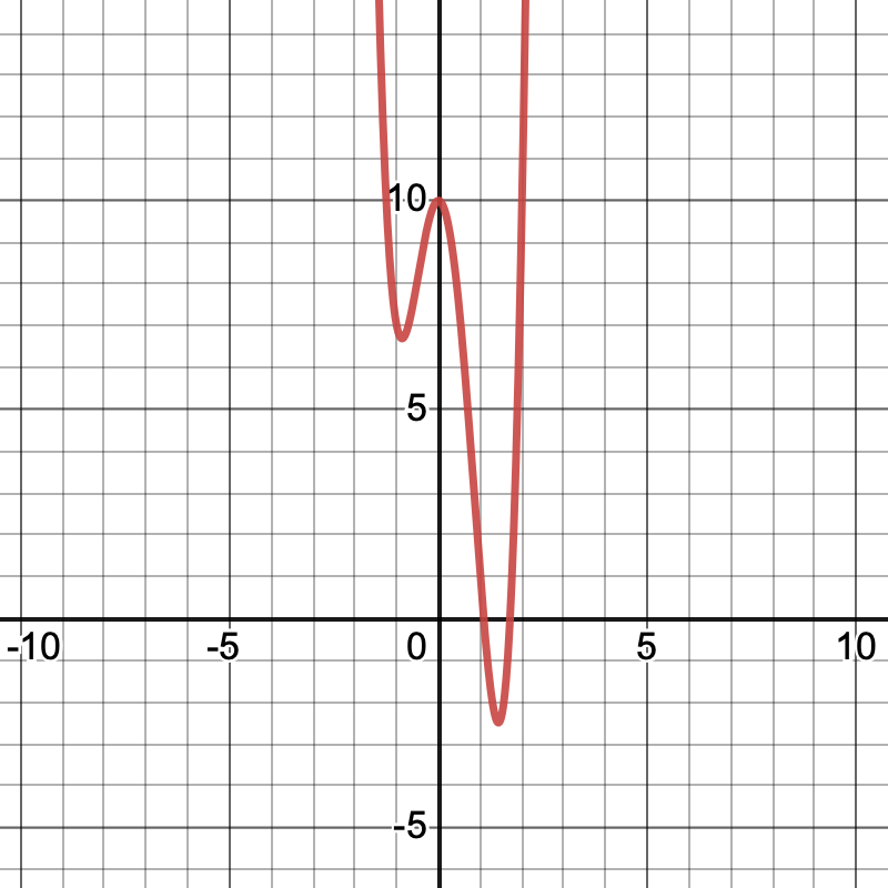
Notice that this function has two minima, one near \(x = -1\) and one near \(x = 1.5\).
The one near \(x = 1.5\) is a global minimum, meaning that it’s the point where the function is the very lowest over all of \(\mathbb{R}.\)
On the other hand, the minimum near \(x = -1\) is a local minimum. We still call it a minimum, but it’s only a minimum relative to the \(x\) that are near it.
When using the gradient descent algorithm on functions like this, what can often happen is that the choice of \(x_0\) and \(t_k\) cause the algorithm to converge to a local minimum rather than a global minimum. In a sense, the algorithm “gets stuck” in a local minimum trough and cannot get out, leading you to believe that the function’s actual minimum point is much higher than it truly is. Testing whether you have obtained the global minimum for a function like \(g\) might be straight forward since \(g\) has only two stationary points; but this can quickly grow into a virtually impossible task when dealing with functions that have hundreds, thousands, or even infinitely many local minima.
On the bright side, one scenario where global optimality is guaranteed is when the gradient descent algorithm converges to a stationary point \(x^*\) of \(f\) (i.e., \(- \nabla f(x^*) = \mathbf{0}\)) and the function \(f\) is convex. We will not cover convex analysis in this article, but suffice it to say that convex functions have the nice property that a point is a local minimum if and only if it is a global minimum. Even so, convex functions are a very small subset of all functions and so in practice, this scenario often doesn’t apply.
A Simple Python Implementation
We’ll now walk through a simple implementation of the gradient descent algorithm in Python. The only package we’ll need to write this implementation is NumPy:
import numpy as np
Next, we’ll write a function that takes each required piece of information as an input and returns the optimal solution and value. More precisely, our gradient descent function should take the following as arguments:
- an objective function
- the gradient of the objective function
- \(x_0\), the starting point
- \(t\), the step size
- \(\epsilon\), the convergence criterion
- a maximum iteration cutoff
Here is the code for my implementation:
def gradient_descent(obj, drvtv, x0, t, epsilon, max_iter):
    # Initialize the algorithm
    x = x0

    # Initialize the iteration counter so that we can stop the
    # algorithm if it doesn't converge within the maximum number of
    # iterations we specify.
    iter_count = 0

    # Start the loop; we want the loop to continue while the
    # convergence criterion is not met. In this case, that's when
    # conv_cond > epsilon. We also have the max_iter argument that
    # will stop the loop even if the convergence criterion hasn't
    # been met. This is useful in practice because sometimes even
    # the convergence criterion we set will never be met and so
    # we want the algorithm to stop if it's been working too long.
    while conv_cond > epsilon and iter_count <= max_iter:
        grad = -drvtv(x)
        prior = x
        x = x + t * grad
        conv_cond = np.linalg.norm(x - prior)
        iter_count += 1

    # Once the loop is finished, we can obtain the objective
    # function's optimal value.

    value = obj(x)

    # Let's print some results. First, we'll say whether the
    # algorithm successfully converged.
    if iter_count > max_iter:
        print("Algorithm did not converge.")
    else:
        print(f"Algorithm converged in {iter_count} iterations.")

    # Finally, we can print the final results; the optimal solution
    # that the algorithm found and the value of the objective
    # function at that optimal solution.
    print(f"\nThe optimal solution was at x = {x}. The objective
        function's value at this point is {value}.")

    return x, value
Let’s test gradient_descent() on the functions we used as examples earlier. As a reminder, those functions were
Python Implementation Example #1
To run gradient_descent() on \(f\), we need to define \(f\) and \(f'\) in the script and then use those functions as arguments in the gradient_descent() function.
def obj1(x):
    return x ** 2 - 2 * x - 3

def drvtv1(x):
    return 2 * x - 2

# Similar to when we ran through this example by hand above, we'll
# initialize the algorithm at x = 3. We'll also choose the same
# stepsize of t = 0.25, but we're going to use a much smaller epsilon
# of 0.0000001 since we can make the computer do all the work now.
gradient_descent(obj = obj1, drvtv = drvtv1,
                 x0 = 3, t = 0.125,
                 epsilon = 0.0000001, max_iter = 1000)
This code returns the following output in the console:
Algorithm converged in 25 iterations.

The optimal solution was at x = 1.0000000596046448. The objective
function's value at this point is -3.9999999999999964.
These are the results we want! The algorithm has returned an optimal solution that is extremely close to what we know is the true optimum value (the optimal solution was \(x = 1\) and the objective function’s value at that point was \(-4\)).
Python Implementation Example #2
To illustrate the problem of getting caught in a local minimum trough, let’s run gradient_descent() on \(g(x)\) twice. The first time, we’ll run it with \(x_0 = 5\) which is greater than the optimal solution. Then, we’ll run it with \(x_0 = -5\) which is less than the non-optimal local minimum and see what results we get.
For both of these runs, we’ll use \(t = 0.001\) and \(\epsilon = 0.0000001\). Here is the code and output for \(x_0 = 5\):
def obj2(x):
    return 4 * (x ** 4) - 3 * (x ** 3) - 10 * (x ** 2) + 10

def drvtv2(x):
    return 16 * (x ** 3) - 9 * (x ** 2) - 20 * x

gradient_descent(obj = obj2, drvtv = drvtv2,
                 x0 = 5, t = 0.001,
                 epsilon = 0.0000001, max_iter = 1000)
This run produces the following output:
Algorithm converged in 232 iterations.

The optimal solution was at x = 1.4341184539432443. The objective
function's value at this point is -2.495603877032643.
By starting somewhere near the true optimum, we obtained a solution that is extremely close to that optimal point (the true optimum is achieved at around \(x \thickapprox 1.4341167\) and the value of \(g\) at that point is about \(-2.4956039\)). But how does the algorithm behave when we start farther away and with a local minimum standing in the way of the true optimum?
Here is the code and output for \(x_0 = -5\):
gradient_descent(obj = obj2, drvtv = drvtv2,
                 x0 = -5, t = 0.001,
                 epsilon = 0.0000001, max_iter = 1000)
This code produces the following output:
Algorithm converged in 363 iterations.

The optimal solution was at x = -0.8716196214233466. The objective
function's value at this point is 6.69805749053783.
So the algorithm still converged but it converged to a point nowhere near the true optimum value. This is precisely because the algorithm fell into the local minimum trough. (the local minimum is at around \(x \thickapprox -0.8716167\) and the value of \(g\) at the point is about \(6.6980575\)) Clearly then, the choice of \(x_0\) is very important when dealing with nonconvex functions.
Python Implementation Example #3
Throughout this article, we’ve only considered the application of the algorithm to single variable functions, but this algorithm really shines when dealing with functions of multiple variables. To illustrate this, let’s consider the following function:
\[h(x, y) = 2x^4 + y^2 - 3xy.\]This function has two global minima at \((x, y) = (3/4, 9/8)\) and \((x, y) = (-3/4, -9/8)\). At both of these points, the value of \(h\) is \(-81/128\) (you can see a visualization of this function here).
We can extend the implementation of the algorithm to handle multivariate functions like this one. To run gradient_descent() on a multivariate function, we just need to modify the objective and derivative arguments to use NumPy arrays.
One thing to keep in mind when we are optimizing multivariate functions is that the derivative is now a gradient. The gradient of a function is the vector of partial derivatives with respect to each of its inputs. For this example, the gradient of \(h\) is denoted and given by
\[\nabla h(x) = \left[ \begin{array}{r} \frac{\partial h}{\partial x} \\\ \\\ \frac{\partial h}{\partial y} \end{array} \right] = \left[ \begin{array}{r} 8x^3 - 3y \\\ \\\ 2y - 3x \end{array} \right].\]Now, we can write the objective function and gradient function so they can be used with gradient_descent().
# The objective function needs to accept a NumPy array instead of
# just one number. Then, we can break the array into its components
# and plug those into the function to get the function's value.
# We'll do this for both the objective function and its gradient.
def obj3(arr):
    x = arr[0]
    y = arr[1]
    return 2 * x ** 4 + y ** 2 - 3 * x * y

def drvtv3(arr):
    x = arr[0]
    y = arr[1]
    partial_x = 8 * x ** 3 - 3 * y
    partial_y = 2 * y - 3 * x
    return np.array([partial_x, partial_y])

init_pos = np.array([0.001, 0.001])
init_neg = np.array([-0.001, -0.001])

gradient_descent(obj = obj3, drvtv = drvtv3,
                 x0 = init_pos, t = 0.01,
                 epsilon = 0.0000001, max_iter = 2000)

gradient_descent(obj = obj3, drvtv = drvtv3,
                 x0 = init_neg, t = 0.01,
                 epsilon = 0.0000001, max_iter = 2000)
This code returned the following output:
Algorithm converged in 1225 iterations.

The optimal solution was at (x, y) = [0.74999816 1.1249925 ]. The objective function's value at this point is -0.6328124999622631.

Algorithm converged in 1225 iterations.

The optimal solution was at (x, y) =  [-0.74999816 -1.1249925 ]. The objective function's value at this point is -0.6328124999622631.
Both of these points are very close to the actual global minima described above and so these are exactly the results we wanted!
Conclusion
To summarize, the gradient descent algorithm is a powerful optimization tool for any ML developer’s toolkit. It has clear computational efficiency advantages and is particularly effective when applied to functions that are convex. Its primary limitation is that we often cannot guarantee that the algorithm will converge to a global optimum. In those instances, it may be better to look at other optimization techniques first to make an informed decision about the best approach.
In future articles, we’ll discuss the Stochastic Gradient Descent algorithm used in machine learning as well as different methods of determining the step size \(t_k\) that can help us guarantee the algorithm’s convergence.